







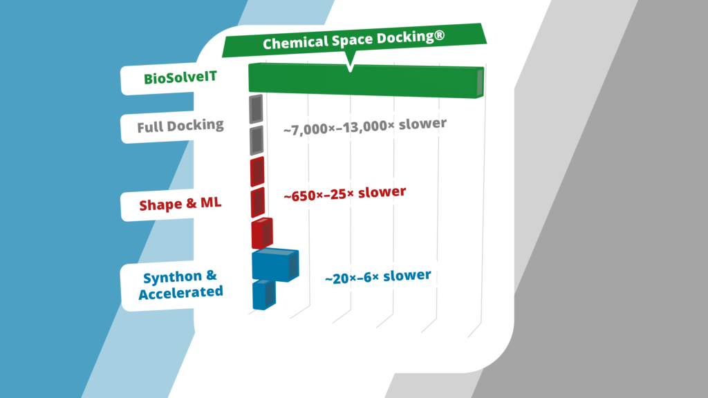

Chemical Space Docking® (C-S-D) is designed for computationally efficient structure-based exploration of ultra-large Chemical Spaces.
But how does it compare with other approaches?
When searching ultra-large Chemical Spaces, computational efficiency and algorithmic strategies are crucial if trillions of compounds are to be screened for potential candidates. The approaches used to tackle this challenge can differ fundamentally: machine learning, combinatorial build-up strategies such as C-S-D, or brute-force docking supported by massive computing resources.
In this article, we examine reported screening campaigns involving ultra-large compound collections and compare their performance with BioSolveIT technologies.
3D Methods
Structure-based 3D methods evaluate molecular candidates based on predicted interactions within the target’s binding site. Favorable interactions are reflected in better scores, which are then used to rank compounds and identify the most promising candidates.
In general, the number of docking calculations that must be performed is the main speed-limiting factor and is ultimately constrained by the available hardware. Combinatorial approaches, such as placing synthons first and subsequently building up complete molecules within the binding pocket, can reduce the required computational effort substantially. Unpromising candidates are eliminated early, leaving only a small fraction of more promising candidates for further evaluation.
The tables below compare C-S-D with other approaches used for screening ultra-large compound collections.
How Does C-S-D Compare to Other Ultra-Large Screening Approaches?
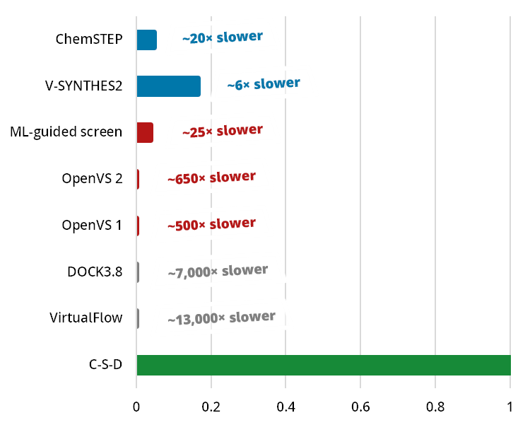
Figure 1. Comparison of 3D search methods applied to ultra-large compound collections. All search performances were normalized to the fastest method, Chemical Space Docking® (C-S-D). In grey: full-library and multistage docking campaigns (brute-force docking). In red: shape- and machine-learning-guided campaigns. In blue: other synthon- and chemical-distance-based accelerated workflows.
Summary: C-S-D represents approximately 5.35 million nominal Chemical Space products per allocated core-hour. Based on the available figures, this is approximately 6× higher than V-SYNTHES2 and 20× higher than ChemSTEP when ChemSTEP similarity traversal and molecular building/docking are combined.
Comparison based on nominal collection size, explicitly processed representatives, and reported or derivable computational expenditure.
| Campaign | Nominal collection | Explicit docking evaluations | Core-hours used | Nominal compounds represented per core-hour | Relative to C-S-D | Training or pre-screening context |
| C-S-D Benchmark | ||||||
| C-S-D PKA / REAL Space |
76 × 109 | 10.67 × 10⁶ | 14,204 | 5.4 × 10⁶ | 1.00× | No machine learning. Includes anchoring, two extension stages, coordinate generation, docking, scoring, and annotation using 288 CPU cores. |
| Full-Library and Multistage Docking Campaigns | ||||||
| Gorgulla et al. VirtualFlow / KEAP1 |
1.3 × 10⁹ | ~1.3 × 10⁹ | ~3–4.5 × 10⁶ | ~300–420 | ~13,000× slower | The complete collection was explicitly docked. The core-hour estimate covers first-stage docking; higher-accuracy rescoring costs are excluded. |
| Liu et al. AmpC |
1.7 × 10⁹ | 1.7 × 10⁹ | 2 × 10⁶ | ~800 | ~7,000× slower | Full-library DOCK3.8 calculation. The reported core-hours cover docking but not necessarily every downstream campaign operation. |
| Shape- and Machine-Learning-Guided Campaigns | ||||||
| Zhou et al. OpenVS / KLHDC2 |
5.5 × 10⁹ | ~6 × 10⁶ | ≤500,000 | ≥11,000 | ~500× slower | Initial docking calculations supplied training and testing data, followed by iterative docking, neural-network retraining, and full-space inference. |
| Zhou et al. OpenVS / NaV1.7 |
4.1 × 10⁹ | ~4.5 × 10⁶ | ≤500,000 | ≥8,100 | ~650× slower | The active-learning workflow stopped after seven iterations. The maximum allocation includes docking, training, prediction, and iterative selection. |
| Luttens et al. ML-guided screen, per target |
3.5 × 10⁹ | 6 × 10⁶ | ~18,000 | ~270,000 | ~25× slower | The first compute block includes docking the training set, model training, and prediction across the nominal collection; final docking adds another 10,344 core-hours. |
| Synthon- and Chemical-Distance-Based Accelerated Workflows | ||||||
| Sadybekov et al. Original V-SYNTHES |
11 × 109 | ~2 × 10⁶ | Not reported | Not calculable | Not calculable | No machine learning. A Minimal Enumeration Library was docked first, followed by iterative enumeration and docking of selected products. |
| Nazarova et al. V-SYNTHES2 |
36 × 109 | 3.8 × 10⁶ | 38,400 | ~940,000 | ~6× slower | No machine learning. CapSelect selects productive MEL poses before hierarchical enumeration and docking of a reduced set of complete products. |
| Mailhot et al. ChemSTEP / AmpC |
13 × 109 | likely ~4.4 × 10 | ~45,000 | ~290,000 | ~20× slower | No machine-learning training. The estimate combines iterative chemical-similarity traversal with molecular building and docking of approximately 0.033% of the nominal collection. |
| Calculation basis: Nominal compounds represented per core-hour = nominal collection size ÷ reported or derived total core-hours. For example, C-S-D represents 76 billion nominal products using an upper-bound allocation of 14,204 core-hours, corresponding to approximately 5.35 million nominal products per core-hour. For V-SYNTHES2, 36 billion nominal products divided by 38,400 CPU-hours gives approximately 937,500 nominal products per core-hour. For ChemSTEP, 13.2 billion nominal products divided by the combined estimate of approximately 45,467 core-hours gives approximately 290,000 nominal products per core-hour.
Important: This metric describes how much nominal library or Chemical Space is represented by the computational workflow per core-hour. It is not a literal rate of complete molecules individually generated, docked, or scored. Accelerated synthon-, similarity-, shape-, and machine-learning-based methods explicitly process only selected representative subsets, while brute-force campaigns dock most or all compounds individually. The campaigns use different docking engines, scoring functions, sampling depths, protein targets, molecular representations, filtering rules, hardware generations, and definitions of total compute. The values therefore provide computational context rather than a controlled head-to-head benchmark. Full methodological details are available in the linked publications. |
||||||
How Does C-S-D Compare to Thompson Sampling Approaches?
Thompson sampling approaches reduce the computational burden of ultra-large virtual screening by docking only a selected subset of compounds. The results from these calculations are used to iteratively update a predictive model, which then prioritizes increasingly promising regions of the compound collection for subsequent evaluation.
This strategy can substantially lower the number of required docking calculations compared with brute-force screening. However, its efficiency depends on the quality of the sampled compounds, the predictive performance of the model, and the number of iterations needed to identify relevant chemistry.
C-S-D follows a fundamentally different principle. Instead of learning from sampled full molecules, it evaluates smaller synthons and progressively assembles promising compounds directly within the binding site. The comparison below examines how efficiently these two approaches navigate ultra-large compound collections relative to the computational resources used.
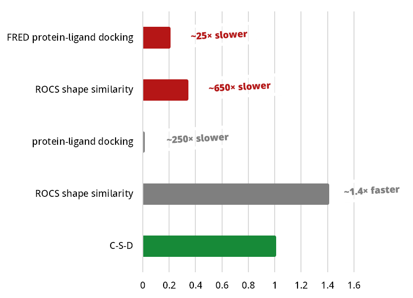
Figure 2. Comparison of C-S-D to Thompson sampling campaigns. All search performances were normalized to Chemical Space Docking® (C-S-D). In grey: original Thompson sampling benchmarks. In red: enhanced sampling and parallelization benchmarks.
Summary: For structure-based screening, C-S-D represents approximately 5.35 million nominal Chemical Space products per allocated core-hour. This is approximately 250× higher than the original Thompson-sampling docking benchmark and approximately 3–5× higher than the later RWS/FRED docking benchmark. Results for 2D similarity and 3D shape searching are included for context but are not directly comparable to docking.
Comparison based on nominal collection size divided by reported or derivable CPU core-hours.
| Campaign | Search objective | Nominal collection | Explicitly evaluated | CPU usage | Nominal compounds represented per core-hour | Relative to C-S-D | Interpretation |
| C-S-D Reference Benchmark | |||||||
| C-S-D PKA / REAL Space |
Structure-based Chemical Space Docking | 76 × 109 | 10.7 × 10⁶ | 14,204 core-hours | 5.4 × 10⁶ | 1.00× | Complete workflow allocation including anchoring, extension, coordinate generation, docking, scoring, and annotation. |
| Original Thompson-Sampling Benchmarks | |||||||
| Klarich et al. Thompson sampling |
ROCS 3D shape similarity | 234 × 106 | ~2.3 × 10⁶ | 32 core-hours | 7.3 × 10⁶ | 1.4× faster | Slightly higher nominal-space coverage, but ROCS shape similarity and structure-based docking answer different questions. |
| Klarich et al. Thompson sampling / JNK3 |
Protein–ligand docking | 335 × 106 | ~3.3 × 10⁶ | 16,000 | 21,000 | 250× slower | The closest original structure-based comparison. Thompson sampling recovered more than half of the exhaustive top 100 after evaluating 1% of the library. |
| Enhanced Sampling and Parallelization Benchmarks | |||||||
| Zhao et al. TS/RWS parallel benchmark |
ROCS 3D shape similarity | 100 × 106 | 200,000 | 64 | ~1.6 × 10⁶ | 3× slower | Near-linear CPU scaling was achieved, although this remains a shape-similarity rather than docking comparison. |
| Zhao et al. TS/RWS parallel benchmark |
FRED protein–ligand docking | 100 × 106 | 200,000 | ~80–115 | ~0.9–1.2 × 10⁶ | ~5× slower | The closest newer docking comparison. The range reflects reduced parallel efficiency when moving from one to 64 CPU cores. |
| Calculation basis: Nominal compounds represented per core-hour = nominal collection size ÷ reported or derivable CPU core-hours. For C-S-D, 76 billion nominal products divided by an upper-bound allocation of 14,204 core-hours gives approximately 5.35 million nominal products per core-hour.
Important: This metric measures the nominal size of the collection addressed by a workflow relative to its CPU allocation. It does not mean that every nominal product was individually generated, docked, or scored. Thompson sampling, RWS, SALSA, and C-S-D explicitly evaluate selected representatives and infer or construct coverage of the remaining combinatorial space. The rows are not controlled head-to-head benchmarks. ROCS shape comparison, FRED docking, and C-S-D use different molecular representations, scoring costs, targets, sampling depths, and definitions of an evaluation. Comparisons are most meaningful between the structure-based docking rows. |
|||||||
2D Methods
Searching ultra-large Chemical Spaces requires methods that can identify relevant compounds without enumerating every possible product. The following comparison places established 2D ligand-based navigation approaches, including fingerprint similarity, MCS and substructure searching, alongside probabilistic Thompson sampling. To provide a consistent performance reference, all reported runtimes are normalized to SpaceLight with ECFP4.
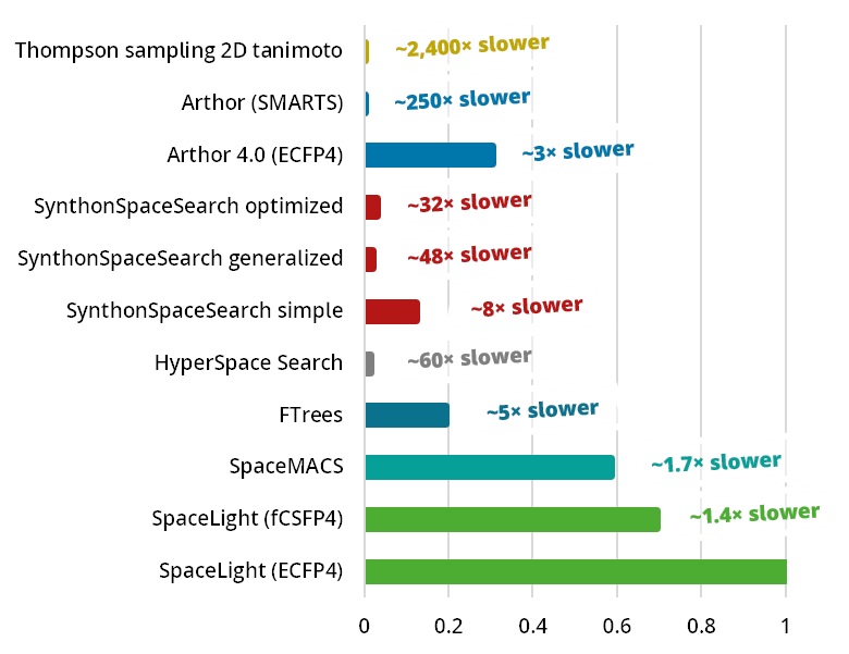
Figure 3. Comparison of 2D search methods applied to ultra-large compound collections. The BioSolveIT methods SpaceLight, SpaceMACS and FTrees are presented at the bottom. As the fastest method, SpaceLight performance was used as reference for the benchmark set of 2,917 compounds and runtimes of all other methods were normalized to it.
Summary: SpaceLight ECFP4 has the lowest reported or extrapolated runtime among the examples included here. Because the results originate from different benchmarks, they provide runtime context rather than a controlled ranking. Based on the reported wall-clock runtimes, it is approximately 1.4× faster than SpaceLight with fCSFP4, 1.7× faster than SpaceMACS, 5.1× faster than FTrees, and approximately 2,440× faster than the reported ligand-based Thompson-sampling benchmark.
Comparison based on the reported or derived wall-clock time required to process 2,917 queries. SpaceLight with ECFP4 is normalized to 1.00×.
| Method | Search objective | Runtime per query | Runtime for 2,917 queries | Relative to SpaceLight (ECFP4) |
| BioSolveIT Ligand-Based Chemical Space Navigation | ||||
| SpaceLight ECFP4 fingerprint similarity |
Fast analog and nearest-neighbor searching | 0.031 s | 1 min 31 s | 1.000× |
| SpaceLight fCSFP4 fingerprint similarity |
Analog searching with a Chemical Space-specific fingerprint | 0.045 s | 2 min 11 s | ~1.4× slower |
| SpaceMACS MCS and motif similarity |
Core, motif, and substitution-pattern searching | 0.053 s | 2 min 35 s | ~1.7× slower |
| FTrees Feature Tree similarity |
Pharmacophore-oriented scaffold hopping | 0.160 s | 7 min 47 s | ~5× slower |
| Other Chemical Space Search Methods | ||||
| Arthor 4.0 ECFP4 fingerprint similarity |
Fingerprint-based similarity searching | ~0.102 s | 4 min 58 s | ~3× slower |
| SynthonSpaceSearch simple substructure query |
Simple substructure searching in synthon spaces | ~0.25 s | 12 min 9 s | ~8× slower |
| SynthonSpaceSearch optimized implementation |
Optimized substructure-oriented synthon searching | ~1.01 s | 49 min | ~32× slower |
| SynthonSpaceSearch generalized substructure query |
Generalized and more complex substructure searching | ~1.50 s | 1 h 13 min | ~48× slower |
| HyperSpace Search Chemical Space searching |
Navigation of combinatorial Chemical Spaces | ~2.0 s | 1 h 37 min | ~60× slower |
| Arthor SMARTS substructure query |
SMARTS-based structural pattern searching | ~8.0 s | 6 h 29 min | ~250× slower |
| Ligand-Based Probabilistic Sampling | ||||
| Klarich et al. Thompson sampling / 2D Tanimoto |
Probabilistic optimization of fingerprint similarity | 1 min 16.2 s | ~61 h 45 min | ~2,400× slower |
| Calculation basis: Relative performance = Runtime of the respective method SpaceLight ECFP4 runtime ÷.
Important: The rows do not represent a controlled head-to-head benchmark. The methods were evaluated using different query sets, nominal collection sizes, hardware configurations, search objectives, result limits, and reporting conventions. Fingerprint similarity, MCS searching, scaffold hopping, SMARTS matching, and probabilistic sampling also address different chemical questions. The Thompson-sampling benchmark evaluated 100,000 products from an approximately 94-million-product library and reported approximate rather than exhaustive top-result recovery. Comparisons should therefore be interpreted as indicative runtime context rather than definitive algorithmic rankings. |
||||
Summary
Taken together, the available benchmarks show that BioSolveIT technologies can navigate ultra-large compound collections and combinatorial Chemical Spaces with high computational efficiency. SpaceLight delivers particularly short runtimes for ligand-based searching, while Chemical Space Docking achieves strong nominal-space coverage per allocated core-hour in structure-based screening. Because the compared studies differ in hardware, datasets, search objectives, and reporting conventions, the results should be interpreted as performance context rather than as a fully controlled head-to-head benchmark.
Further detailed insights can be found on our FAQs page.